UPDATE 30 May 2018: See latest post for online deployment of the models presented here
UPDATE 25 May 2018: See following post for refinements to the models presented here
This is the next in the series of my Artificial Intelligence (AI) / Machine Learning (ML) posts . The
first covered the use of TensorFlow for Object Detection. The
second described how to deploy the trained TensorFlow model on the Google Cloud ML Engine.
In this third post, I focus entirely on
MATLAB in order to explore its machine learning capabilities, specifically for prototyping ML models. The topic of deploying the trained models for production is touched upon but not expanded here.
As in my previous posts, I make no apologies for any technical decisions which may be considered sub-optimal by those who know better. This was an AI/ML learning exercise for me, first and foremost.
The Goal
Devise an ML algorithm to forecast the (aviation) weather, in half-hour increments, up to three days into the future, using historical time series of weather data. I was motivated to tackle this specific problem because (i) high-quality aviation weather data is readily available -- so the task of data preparation and cleansing is minimised, enabling the focus to be primarily on the ML algorithms; (ii) I've lamented the loss of the (very useful -- in my opinion) 3-day aviation forecast from the UK MET Office website ever since they removed it a couple of years ago.
The Dataset
For this initial exploration, I used aviation weather data (
METARs) for Ronaldsway Airport (EGNS) on the Isle of Man since (i) I am based here and fly my Scottish Aviation Bulldog from here; (ii) being located in Northern Europe, the weather is varied and changeable, so the models (hopefully) have interesting features to be detected during training, thereby exercising the models' forecasting capabilities more than if the weather was uniform and more easily predictable. The modelling techniques presented for this single location can of course be extended to any other location for which analogous data exists (i.e., pretty-much anywhere).
The underlying weather data was obtained from
US NOAA/NWS (as utilised in
JustMET,
iNavCalc, and
ReallySimpleMovingMap). The training set comprised METAR data captured every half hour for EGNS over the 3.5 month period from 30 December 2017 through 13 April 2018. Each half-hourly recorded METAR was persisted (for long term storage e.g., for future analysis) to an
Amazon DynamoDB database, as well as to a
Microsoft Azure SQL database (for temporary storage and staging). The triggering to capture each successive half-hourly METAR via web-service calls to NOAA was implemented using a
Microsoft Azure Scheduler.
The Toolkit
Solution Path
Pre-processing the Raw Data
The first task was to pre-process the raw data, in this case, primarily to correct for data gaps since there was (inevitably) some (unforeseen) down-time over the weeks and months in the automated METAR capture process.
To start out, the data was retrieved (into MATLAB) from the Azure SQL database using the MATLAB Database Toolbox functionality.
GOTCHA: the graphical interface bundled with the MATLAB Database Toolbox is rather limited and cannot handle stored procedures. Instead, the command-line functions must be used when retrieving data from databases via stored-procedures.
Next, the retrieved data was reformatted into a MATLAB
Timetable. This proved to be a very convenient format for manipulating and preparing the data. It is an extension of the MATLAB
table format, designed specifically to handle time-stamped data, and therefore ideal for handling the multivariate METAR time-series. Note: the MATLAB
table format is a relatively recent innovation, and seems to be MATLAB's answer to the
DataFrame object from the powerful and popular
pandas library available for Python.
The set of 8 variables collected for analysis and forecasting are summarised below (for detailed definitions, see
here). The variables pertain to observations made on the ground at the location of the given weather station (airport), distributed via the METAR reports. I have kept the units as per the METARs (rather than converting to S.I.). Each observation (i.e., at each sample time) contains the following set of data:
- Temperature (units: degrees Celsius)
- Dewpoint (units: degrees Celsius)
- Cloudbase (units: feet)
- Cloudcover (units: oktas, dimensionless, 0 implies clear sky, 8 implies overcast), converted to numerical value from the raw skycover categorical variable from the METAR (i.e.,"CAVOK" -- 0 oktas; "FEW" -- 1.5 oktas; "SCT" -- 3.5 oktas; "BKN" -- 5.5 oktas; "OVC" -- 8 oktas). Note: whenever "CAVOK" was specified, this was taken to set the Cloudcover value to zero and the Cloudbase value to 5000 feet -- even if skies were clear all the way up since the METAR vertical extent formally ends at 5000 feet above the airport (typically). Making this assumption (hopefully) means erring on the safe side, even if it tampers -- in a sense --with the natural data.
- Surface Pressure (units: Hectopascals)
- Visibility (units: miles)
- Wind Speed (units: knots)
- Wind Direction (units: degrees from True North)
Additionally, the date and time of each observation is given (in UTC), from which the local time-of-day can be determined from the known longitude via the MATLAB expression:
timeofday=mod(timeutc+longitude*12/180,24);
Note: as well as local-time-of-day, it would also be worthwhile to include the day-of-year in the analyses (since weather is known to be seasonal). This was not done for now since the entire data set spans only 3.5 months rather than at least one complete year. This means that since the validation set is taken from the 30% tail-end (see later), and the training set is the 70% taken from the start, up to the beginning of the tail-end, there will be no common values for day-of-year in both the training and validation sets, so it is not sensible to include day-of-year for now. However, if/when the collected data set spans sufficient time (1.3 years for the 30:70 split) such that the training and validation sets both contain common values for day-of-year, then it should be included in a future refinement.
Filling the Data Gaps
The MATLAB command for creating the aforementioned
timetable structure from individual vectors is as follows:
TT=timetable(datetimeUTC,temperature,dewpoint,cloudbase,
cloudcover,visibility,sealevelpressure,windspeed,...
winddirection,timeofday);
Since all the variables in the
timetable are continuous (rather than categorical), it is simple in MATLAB to fill for missing data by interpolation as follows:
% Define the complete time vector, every 30 minutes
newTimes = [datetimeUTC(1):minutes(30):datetimeUTC(end)];
% Use interpolation for numerical values
TT.Properties.VariableContinuity = {'continuous','continuous','continuous','continuous',...
'continuous','continuous','continuous','continuous',...
'continuous'};
% Perform the data filling
TT1 = retime(TT,newTimes);
METAR Data Time Series Plots
These cleaned METAR time series for EGNS are plotted in the graphs below and serve as the source of training and validation data for the upcoming ML models. Each time series is 4,974 data points in length (corresponding to the 3.5 month historical record, sampled each half hour).
Modelling Phase 1: LSTM models for each variable
Since it is generally known that long short-term (LSTM) neural networks are well-suited to the task of building regression models for time series data, it seemed the natural starting point for these investigations, not least since
LSTM layers are now available within MATLAB.
A separate LSTM model was therefore built for each of the METAR data variables by following the MATLAB example presented
here. Note: it is possible to build an LSTM model for multiple time series taken together, but I felt it would be "asking too much" of the model, so I opted for separate models for each (single variable) time series. It may be worthwhile revisiting this decision in a future attempt at refining the modelling.
When building the models for the METAR data, the various (hyper-)parameters available within the LSTM model for "tweaking" (such as the number of neurons, per layer the number of layers, the number of samples back in time to be used to fit the model for looking forward in time, etc) not surprisingly needed to be changed from the default settings and from those settings presented in the
MATLAB example, in order to achieve useful results on the METAR data. This is not unreasonable, given that the data sets are so different, and that machine learning is essentially data-driven. By trial-and-error experimentation, the following code snippet captures the set of hyper-parameters which were found to be effective on the METAR variables.
%% Example data setup for LSTM model on the first chunk of data
% Look back 92 hours. Seems suitable for METAR data
numTimeStepsTrain = 184;
% 3 days maximum forecast look-ahead
numTimeStepsPred = 144;
windowLength = numTimeStepsPred+numTimeStepsTrain;
data=data_entire_history(1:windowLength);
% where data_entire_history is entire time series
XTrain = data(1:numTimeStepsTrain);
% where data is the first window of time series
YTrain = data(2:numTimeStepsTrain+1);
% target for LSTM is one time-step into the future
XTest = data(numTimeStepsTrain+1:end-1);
% inputs for testing the LSTM model at all forecast look-aheads
YTest = data(numTimeStepsTrain+2:end);
% targets for testing the LSTM model at all forecast look-aheads
%For a better fit and to prevent the training from diverging,
%standardize the training data to have zero mean and unit variance.
%Standardize the test data using the same parameters as the training
%data.
mu = mean(XTrain);
sig = std(XTrain);
XTrain = (XTrain - mu) / sig;
YTrain = (YTrain - mu) / sig;
XTest = (XTest - mu) / sig;
%% Define LSTM Network Architecture
inputSize = 1;
numResponses = 1;
numHiddenUnits =65; % seems suitable for METAR data
layers = [ ...
sequenceInputLayer(inputSize)
lstmLayer(numHiddenUnits)
fullyConnectedLayer(numResponses)
regressionLayer];
maxEpochs=200;
opts = trainingOptions('adam', ...
'MaxEpochs',maxEpochs, ...
'GradientThreshold',1, ...
'InitialLearnRate',0.005, ...
'LearnRateSchedule','piecewise', ...
'LearnRateDropPeriod',125, ...
'LearnRateDropFactor',0.2, ...
'Verbose',0);
% Train the LSTM network with the specified training options by
% using trainNetwork.
net = trainNetwork(XTrain,YTrain,layers,opts);
% Forecast Future Time Steps
% To forecast the values of multiple time steps in the future,
% use the predictAndUpdateState function to predict time steps
% one at a time and update the network state at each prediction.
% For each prediction, use the previous prediction as input to
% the function.
% To initialize the network state, first predict on the training
% data XTrain. Next, make the first prediction using the last
% time step of the training response YTrain(end). Loop over the
% remaining predictions and input the previous prediction to
% predictAndUpdateState.
net = predictAndUpdateState(net,XTrain);
[net,YPred] = predictAndUpdateState(net,YTrain(end));
numTimeStepsTest = numel(XTest);
for i = 2:numTimeStepsTest
[net,YPred(1,i)] = predictAndUpdateState(net,YPred(i-1));
end
% Unstandardize the predictions using mu and sig calculated
% earlier.
YPred = sig*YPred + mu;
% The training progress plot reports the root-mean-square error
%(RMSE) calculated from the standardized data. Calculate the RMSE
% from the unstandardized predictions.
rmse = sqrt(mean((YPred-YTest).^2))
Note: it may be better to tweak the hyper-parameters specific to the modeling of each variable, again, not done, here, but an idea for future enhancements.
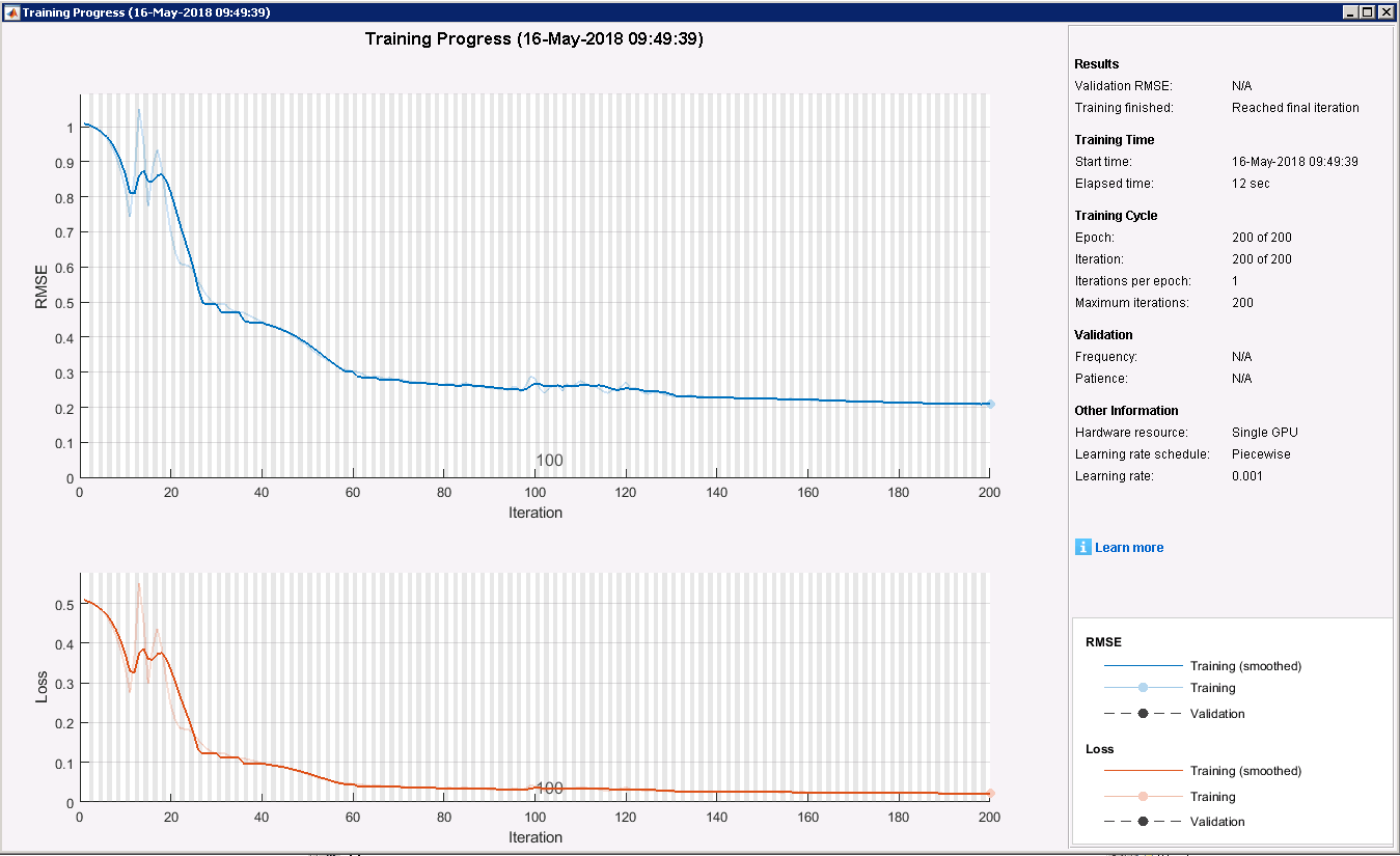
Using the above-mentioned set of hyper-parameters, the graph below shows a typical LSTM training convergence history (in this case, for Temperature). Note: this plot, (optionally) generated by MATLAB interactively during training, is similar to that available via
TensorBoard (when training TensorFlow models), but with the added advantage that there is a "Stop Button" on the MATLAB interface that enables the user to stop the training at any time (and capture the network parameters at that time).
The typical forecast results (i.e., from just one arbitrary window of the historical data set) obtained from the LSTM models for each variable are shown in the following plots. In each plot, the (92 hour) training data window is (arbitrarily) chosen to be before "time zero" when the forecast starts (and extends from half an hour to 72 hours i.e., 3 days). The black curve is the training data, the blue curve the forecast results, and the red curve the test values against which the forecast performance can be directly compared. For all METAR variables, the forecasts are seen to be effective only out to a few hours at most, with significant deviations beyond that -- and some variables are worse than others.
Forecast Error Plots
By re-training each LSTM model for each METAR variable, at
each successive sample point in the test data set, and comparing with the known measurements for each forecast time, it is possible to build-up a statistical picture of the average performance of the models over forecasting time. For the 3.5 month historical METAR data set, sampled every half hour, and subtracting two window widths (first and last), this implies training approximately 4600 LSTM models per METAR variable. Note: when it comes to production deployment of the models, the principle of re-training each model at each sample point i.e., each time a new weather observation comes in -- every half hour in the case of METARs, --means that the model for the given variable is the most up-to-date that it can be at any given time, for use in forecasting forward from that point in time. By averaging the mean-squared error in the (4600) forecasts of each of the trained models sliding forward in time from the begin to the end of the entire data set, the expected accuracy of the forecast for each look-ahead forecast time can be assessed. These accuracies (in terms of absolute average mean-square error and relative average mean-square error) are plotted in the Forecast Error Plots below (blue curves, labelled "
LSTM alone") for each variable versus look-ahead time (from half an hour to three days). On the absolute error plots, the standard deviation of the underlying observations is also shown (denoted
sdev obs). Whenever the error curve is (well) below the
sdev obs line, the forecast can be considered better than random. But whenever the error curve is near to or above the
sdev obs line, the forecast is no better than random, and should be considered as ineffective. Similarly, on the relative error curves, whenever the error is below 50% (as indicated by the line marked
50% error), the forecast may be considered as effective, though the lower the better. Above a relative error of 50%, the forecast should be considered as ineffective.
In terms of the range to which the LSTM forecasts are considered useful (in terms of look-ahead period), these values have been extracted from the plots and summarised in the following table.
| Variable | Usable forecast |
| Temperature | 6 hours |
| Dewpoint | 2 hours |
| Cloudbase | 2 hours |
| Cloud Cover | No usable forecast |
| Sea-Level Pressure | 25 hours |
| Visibility | 2 hours |
| Windspeed | 3 hours |
| Wind Direction | 3 hours |
The LSTM forecasts are generally seen to be useful out to a few hours, with some exceptions: Sea-Level Pressure forecast is good out to (an impressive) 25 hours; but Cloud Cover forecast is no good at all.
Modelling Phase 2: Using the LSTM model outputs in combination with the other METAR variables to perform regressions
The benefit of the LSTM modelling from Phase 1 above is that the recent history of a given variable is utilised in predicting it's future path. This should presumably be better than using just a single snapshot in time (e.g., now) to predict the future. That said, from the results obtained, the accuracy diminishes quite significantly when forecasting out beyond a couple of hours or so. In this next phase, the idea is to utilise the information from the other METAR variables to help improve the forecasts for the given variable (which so far has been based only on histories of itself). This makes sense from the laws-of-physics point of view. For example, the temperature an hour from now will depend not only on the temperature now, but on: the time of day (since there is a diurnal temperature cycle) of the measurement and of the desired forecast; the extent of cloud cover; the wind strength (possibly), etc., so it makes intuitive sense to somehow tie these other known measurements and time-factors into the forecasts for a given variable.
The strategy therefore is to re-cast the forecasting task as a neural network multivariate regression problem where the inputs (regressors) comprise: (i) all the measured METAR variables at a given time, (ii) the time of day of those measurements, (ii) the time difference between the measurement time and the time of the forecast looking ahead; (iii) and the estimated value of the variable in question at the time of the forecast looking ahead obtained from the LSTM model from Phase 1. The output (target) of the regression is the estimate of the value of the variable in question at the time of the forecast looking ahead (for each look ahead time). For training, all input and output values are known. Moreover, since the LSTM models have been re-defined every half hour (by sliding through the entire data set), a large set (i.e., 664,521) of input/output values is available for training this neural net regression model.
To perform the neural network regression, MATLAB has two options available: the (older) train function; and the newer trainNetwork function (which was used above for the LSTM training). The differences between the two methods are discussed here. I opted to use the newer trainNetwork method since it is focused on Deep Learning and can make use of large data sets running on GPUs. At this point I would like to extend my gratitude to Musab Khawaja at the Mathworks who provided me with sample code (in the snippet below) demonstrating how to adapt the imageInputLayer (normally used for image processing) for use in general-purpose multivariable regression.
As with the LSTM modelling, the hyper-parameters need to be chosen for the training. Again, by trial-and-error, the following common set (within the code snippet below) proved to be suitable for each of the METAR data fits:
% Here, x is the array of appropriate regressor observations, and
% t is the vector of targets
% Create a table with last col the outputs
data=array2table([x' t']);
[sizen,sizem]=size(x);
numVars = sizen;
n = height(data);
% reshape to 4D - first 3D for the 'image', last D for each
% sample
dataArray = reshape(data{:,1:numVars}', [numVars 1 1 n]);
% ...assume first numVars columns are predictors (regressors)
output = data{:,numVars+1}; % assume response is last column
% Split into 70% training and 30% test set
pc = 0.7;
rng('default') % for reproducibility
idx=1:n;
% Don't shuffle yet, since don't want training sliding
% window to leak into validation set
max_i = ceil(n*pc);
idxTrain = idx(1:max_i);
idxTest = idx(max_i+1:n);
% Now shuffle the training and validation sets independently
idxTrain=randsample(idxTrain,length(idxTrain));
idxTest=randsample(idxTest,length(idxTest));
% Prepare arrays for regressions
trainingData = dataArray(:, :, :, idxTrain);
trainingOutput = output(idxTrain);
testData = dataArray(:, :, :, idxTest);
testOutput = output(idxTest);
testSet = {testData, testOutput};
% Define network architecture
layers = [...
imageInputLayer([numVars,1,1]) % Non-image regression!
fullyConnectedLayer(500) % Seems suitable for METAR data
reluLayer
fullyConnectedLayer(100)
reluLayer
fullyConnectedLayer(1)
regressionLayer
];
% Set training options
options = trainingOptions('adam', ...
'ExecutionEnvironment','gpu', ...
'InitialLearnRate', 1e-4, ...
'MaxEpochs', 1000, ...
'MiniBatchSize', 10000,...% Seems suitable for METAR data
'ValidationData', testSet, ...
'ValidationFrequency', 25, ...
'ValidationPatience', 5, ...
'Shuffle', 'every-epoch', ...
'Plots','training-progress');
% Train
net = trainNetwork(trainingData, trainingOutput, layers, options);
% Predict for validation plots
y=predict(net,testData);
VALIDATION_INPUTS=reshape(testData,[numVars,length(testData)])';
VALIDATION_OUTPUTS=testOutput;
VALIDATION_y=y;
A Deep Learning model with the afore-mentioned hyper-parameters was trained for each METAR variable, in turn, selected as the target. As evident from the code snippet, the first 70% of the entire data set was used for training (which amounted to 465,165 data points), the remaining 30% ("tail-end") for validation (which amounted to 199,356 data points).
The errors in the corresponding forecasts when applied to the validation data are displayed as the red curves (labelled "Multi-regression plus LSTM") in the Forecast Error Plots presented earlier. For comparison, the yellow curves (labelled "Multi-regression alone") in the error plots correspond to the multivariate regressions re-trained but this time excluding the LSTM outputs as regressors. It can be seen that in all cases, the LSTM models out-perform the Multi-regressions when limiting our attention to those regimes where the forecasts are deemed to be useful i.e., when the absolute rms error is below the standard deviation of the observations and when the relative rms error is below 50%. This came somewhat as a surprise, since intuitively it was felt that the addition of information via the other variables
should have been more beneficial than was observed. Perhaps a refined regression analysis, as discussed below, would reveal such. Outside the usable regimes, the Multi-regressions sometimes out-perform the LSTM models, but by then, none of the models are effective (errors too large). It is also interesting to note that the inclusion of the LSTM outputs as inputs to the Multi-regressions generally improves their performance (i.e., red curves lower than yellow curves) -- but not in every case (see for example, the Cloudbase forecasts, where the yellow curve is lower than the red curve).
Other Things To Try
Some ideas to try next include (not exhaustive):
- The LSTM models were trained to target the observations just one sample period (half hour) away from the inputs, but then asked to predict out to three days away, with the accuracy dropping off dramatically within the first few samples ahead. Instead, it might be worth trying training a different LSTM model for each look-ahead period (by down-sampling before training). This would entail having a different LSTM model per look-ahead period, but perhaps the forecast accuracy would be better, particularly further out ?
- Likewise, for the Multi-regression models, all look-ahead periods were included in a single regression model. This means that the accuracy for the short look-ahead periods is penalised by the errors further out (since the stochastic gradient descent optimiser minimises a single number: the rms error across all look-ahead periods). Instead, it might be worth trying training a different Multi-regression model for each look-ahead period. Again, this would entail more models, but the accuracy may be better.
- The hyper-parameter settings for all models were set via trial-and-error. It might be worth trying a more systematic approach e.g., by invoking an outer layer of optimisation which uses for example, techniques invoking genetic algorithms, to choose the optimum set of hyper parameters.
- Try incorporating additional information in the regressions. For example, weather data for other locations known to correlate with the weather in the given location. Case-in-point: since most of the weather systems on the Isle of Man originate from the Atlantic i.e., to the west, it might be useful to incorporate weather data from Ireland, with suitable lag, to try and improve the model predictions for the Isle of Man.
End-to-End Recipe For Weather Forecaster
If the Multi-regression results can be improved by the suggestions above, such that they can compete with the LSTM models over some portion(s) of the look-ahead range, then the following general recipe for an online ML-based weather forecaster can be proposed:
Every few months (or so):
- For a given location, gather as long a history of half-hourly METAR data as possible/available, ideally over at least the past year in order to capture seasonal variations
- From the data in 1), perform a set of LSTM fits (sliding across the data, one sample at a time) to obtain the estimated quantities for use as inputs (alongside the METAR data) to the multivariate regressions. Note: for the 3.5 month historical data set, this set of fits took approximately two days per METAR variable on a p2.xlarge (GPU-equipped) AWS instance, owing to the many thousands of LSTM training runs required.
- With the data from 1) combined with the estimates from 2), Perform Deep learning multivariate regressions for each target variable. Refer to this trained model as the REGRESSION MODEL for the given target variable. Also perform a regression for the given target variable excluding the LSTM estimates as a regressor. Refer to this trained model as the REDUCED REGRESSION MODELfor the given target variable. Note: for the 3.5 month historical data set, these two fits took approximately one hour per METAR variable on a p2.xlarge (GPU-equipped) AWS instance. Re-create a revised set of Forecast Error Plots from the results of the runs in 2 & 3 (in order to be able to select the best model per forecast look-ahead period, see below).
Every time a new observation is received (half-hourly):
- Re-train the LSTM models, one per variable, using the latest measurement as the most recent available. For each variable, refer to this trained model as the LSTM MODEL for the given variable (note: this fit will take a few minutes per METAR variable on a p2.xlarge GPU-equipped AWS instance).
- For each forecast look-ahead period (i.e., half hourly up to three days ahead), use each LSTM MODEL each REGRESSION MODEL, and each REDUCED REGRESSION MODEL to generate three different forecasts for the given variable (note: these will take only a few seconds per METAR variable on a p2.xlarge GPU-equipped AWS instance). For each forecast look-ahead period, choose the forecast (i.e., from the LSTM MODEL, the REGRESSION MODEL, or the REDUCED REGRESSION MODEL) depending on which gives the lowest rms error for the given forecast look-ahead period, by referring to the updated Forecast Error Plots.
Production Deployment Possibilities
The optimum choice of computational and software platform for the Production Deployment of the end-to-end ML-based weather forecaster presented above is not at all clear, requiring a detailed exploration of the available technical options and trade-offs. However, the following possibilities come to mind, each with its own advantages and disadvantages:
- Deploy on a suite of MATLAB-equipped Cloud-based server instances. Has the advantage that the code can be used essentially "as is" (since the MATLAB code is already written via the prototypes presented here). Has the disadvantage with respect to cost that the servers would have to be "always on", and the associated MATLAB licensing costs may become prohibitive.
- Use the MATLAB compiler to package the trained models into deployable libraries which can be installed within (say, Docker) containers which can be instantiated on-demand in the Cloud (and automatically shut down when dormant). Has the advantages that the code is essentially written (just needs to be run through the MATLAB compiler); and that by using containers, there is no need to incur the cost of "always on" server instances. There some open questions, however: can the (half hourly) re-training of the LSTM models via the trainNetwork function be compiled via the MATLAB Compiler?; can functions deployed from the MATLAB Compiler access GPUs, or must the GPU Coder be used?; can compiled MATLAB software running within containers access GPUs?
- Re-write the models in an open-source ML framework such as TensorFlow and deploy on the Google Cloud ML Engine as exemplified here. Has the disadvantage that all the models would have to be rewritten, outside MATLAB.
- Any suggestions welcome : )
A Note On Workflow
In the past, I would tend to use MATLAB much like I would use other functional programming languages i.e., by creating many functions (subroutines) and calling them from a main program. However, by its very nature, machine learning is much more of a trial-and-error process than the type of analyses I have been used to. It is generally more amenable to the interactive process of defining a set of parameters, running the parameters through a script (e.g., which contains the ML model training commands), viewing the outputs (e.g., in terms of suitable performance metrics), re-assessing the assumptions and tweaking the parameters accordingly, then running the script again, etc., until a satisfactory outcome has been achieved. In fact, this very mode of interaction has resulted in Jupyter Notebooks being one of the most widely-used IDEs for developing ML models in Python. Again, MATLAB seems to have their own recently-introduced answer to this: namely, the MATLAB Live Editor. As such, when starting out on this exploration, and having successfully used Jupyter Notebooks for Python on previous ML projects, I launched into using the MATLAB Live Editor for running the aforementioned interactive ML design scripts. Whilst I found this to be useful in the early prototyping stage for a given model, I reverted back to the tried-and-tested technique of executing scripts (stored in m-files) with embedded local sub-functions (for calling from loops in the given script). I simply found this mode of operation to be more productive. Also, the publish options from Live Edit seemed to be less flexible and less configurable than for normal m-file scripts.
Conclusions
- MATLAB is a highly productive platform for prototyping Machine Learning (in particular, Deep Learning) algorithms. The data-wrangling tools are excellent. In my opinion, it is easier to develop the ML models in MATLAB than in Python/TensorFlow, but that could be due to the fact that I have a long experience (decades) with using MATLAB compared with only a few weeks using Python/TensorFlow.
- Weather forecasting is a hard problem. The Deep Learning approaches developed here show some promise, particularly the LSTM models, but generally only out to a few hours -- and not to the 3 days desired at the outset. Further refinement (perhaps along the lines presented above in Other Things To Try) would hopefully improve the predictive ability of the models.