Deep Learning Analysis of COVID-19 lung X-Rays using MATLAB: Part 3

UPDATES: See Part 4 for a grad-CAM analysis of all the trained networks presented below, then Part 5 where the grad-CAM results of Part 4 are used to train another suite of networks to help choose between the lung X-ray classifiers presented below.

*** DISCLAIMER ***

I have no medical training. Nothing presented here should be considered in any way as informative from a medical point-of-view. This is simply an exercise in image analysis via Deep Learning using MATLAB, with lung X-rays as a topical example in these times of COVID-19. 

INTRODUCTION

In this Part 3 in my series of blog articles on exploring Deep Learning of lung X-rays using MATLAB, the analysis of Part 1 is revisited but rather than just using the pre-trained googlenet as the basis of Transfer Learning, the performance of all the pre-trained networks available via MATLAB as the basis for the Transfer Learning procedure is compared.

AVAILABLE PRE-TRAINED NETWORKS

See this overview for a list of all the available pre-trained Deep Neural Networks bundled with MATLAB (version R2020a). There are 19 available networks, listed below, which include two alternate versions of googlenet: the original, and the alternate version with identical layer structure but pre-trained on images of places rather than images of objects. 

Available Pre-Trained Networks

squeezenet

googlenet

googlenet (places)

inceptionv3

densenet201

mobilenetv2

resnet18

resnet50

resnet101

xception

inceptionresnetv2

shufflenet

nasnetmobile

darknet19

darknet53

alexnet

vgg16

vgg19

TRANSFER LEARNING

Network Preparation

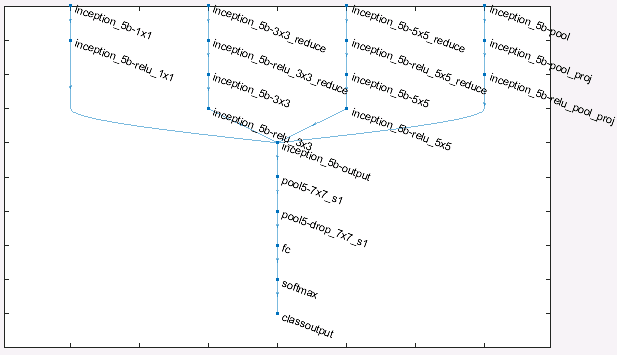
Each of the above pre-trained networks were prepared for Transfer Learning in the same manner as described in Part 1 (and references therein). This involved replacing the last few layers in each network in preparation for re-training with the lung X-ray images. To determine which layers to replace required identifying the last learning layer (such as a convolution2dLayer) in each network and replacing from that point onwards using new layers with the appropriate number of output classes (e.g., 2 or 4 etc rather than 1000 as per the pre-trained imageNet classes). For convenience, I've collected together the appropriate logic for preparing each of the networks (since the relevant layer names are generally different for the various networks) in the function prepareTransferLearningLayers which you can obtain from my GitHub repository here.

Data Preparation

For each of the Examples 1--4 in Part 1,  the training and validation image datasets were prepared as before (from all the underlying images available) with the important additional action: for each Example, the respective datasets were frozen (rather than randomly chosen each time) so that each of the 19 networks could be trained and tested on precisely the same datasets as one another, thereby enabling ready comparison between network performance.

Training Options

The training options for each case were set as follows:

MaxEpochs=1000; % Placeholder, patience will stop well before
miniBatchSize = 10;
numIterationsPerEpoch = floor(numTrainingImages/miniBatchSize);
options = trainingOptions('sgdm',...
  'ExecutionEnvironment','multi-gpu', ...% for AWS ec2 p-class VM
  'MiniBatchSize',miniBatchSize, 'MaxEpochs',MaxEpochs,...
  'InitialLearnRate',1e-4, 'Verbose',false,...
  'Plots','none', 'ValidationData',validationImages,...
  'ValidationFrequency',numIterationsPerEpoch,...
  'ValidationPatience',4);

Note that the ValidationPatience is set to a finite value (e.g., 4 rather than Inf) to automatically halt the training before overfitting occurs. This also enables the training to be performed within a big loop across all 19 network types without user intervention. Also note that ExecutionEnvironment was set to multi-gpu to take advantage of the multiple GPUs available via Amazon Web Services (AWS)  p-class instance types in order to speed-up the analysis for all networks across all examples. The screenshot below shows the GPU activity when running the training on an AWS p2.x8large instance type. Even with GPUs, some training runs took quite a long time, especially for the larger networks (not surprisingly). For example, nasnetlarge on the Example 2 dataset (3434 training images)  took 11 hours to complete.  All in all, it took a few days to complete the training for all 76 cases (i.e., the 4 Example Cases across each of the 19 networks)

Deep Learning Network training via MATLAB on an AWS p2.x8large instance with 8 NVIDIA Tesla GPUs

RESULTS

Refer to Part 1 for the motivation and background details pertaining to the following examples. 

EXAMPLE 1: "YES / NO" Classification of Pneumonia

The 19 networks were re-trained (via Transfer Learning) on the relevant training dataset for the given example (1280 images, equally balanced across both classes). The following table shows the performance of each trained network when applied to the validation dataset (balanced, 112 each "yes" / "no") and the holdout dataset (unbalanced, 3806 "yes" only). The results are ordered (descending) by (i) Average Accuracy (across both classes), then (ii) Pneumonia Accuracy (i.e., fraction of "yes" correctly diagnosed). The table also included the Missed Pneumonia rate i.e., the percentage of the total validation population that should have been diagnosed "yes" (pneumonia) but which were missed i.e., wrongly diagnosed as "no" (healthy).

Base network	Validation: Average Accuracy	Validation: Pneumonia Accuracy	Validation: Healthy Accuracy	Validation: Missed Pneumonia	Holdout: Average Accuracy
vgg16	91%	88%	95%	6%	86%
alexnet	90%	86%	94%	7%	85%
darknet19	88%	88%	88%	6%	87%
darknet53	88%	89%	87%	5%	89%
shufflenet	88%	84%	92%	8%	84%
googlenet	88%	83%	93%	8%	84%
googlenetplaces	88%	89%	86%	5%	87%
resnet101	88%	77%	98%	12%	76%
nasnetlarge	87%	83%	91%	8%	84%
resnet50	87%	86%	88%	7%	88%
vgg19	86%	90%	81%	5%	91%
xception	86%	79%	93%	11%	83%
resnet18	85%	71%	100%	15%	77%
squeezenet	84%	92%	76%	4%	91%
densenet201	83%	71%	96%	15%	72%
inceptionresnetv2	83%	92%	73%	4%	86%
nasnetmobile	72%	84%	60%	8%	85%
inceptionv3	72%	83%	61%	8%	83%
mobilenetv2	69%	93%	46%	4%	93%

EXAMPLE 2: Classification Bacterial or Viral Pneumonia

The 19 networks were re-trained (via Transfer Learning) on the relevant training dataset for the given example (3434 images, equally balanced across both classes). The following table shows the performance of each trained network when applied to the validation dataset (balanced, 320 each "bacteria" / "virus") and the holdout dataset (unbalanced, 520 "bacteria" only). The results are ordered (descending) by (i) Average Accuracy (across both classes), then (ii) Viral Accuracy (i.e., fraction of viral cases correctly diagnosed). Also shown is the Missed Viral rate (i.e., the fraction of the total validation population that should have been diagnosed viral but which were missed (wrongly diagnosed as bacterial).

Base network	Validation: Average Accuracy	Validation: Viral Accuracy	Validation: Bacterial Accuracy	Validation: Missed Viral	Holdout: Average Accuracy
darknet53	80%	76%	84%	12%	84%
vgg16	80%	73%	87%	14%	83%
squeezenet	79%	75%	83%	12%	80%
vgg19	78%	79%	78%	10%	78%
mobilenetv2	78%	81%	75%	9%	71%
googlenetplaces	78%	71%	86%	15%	85%
densenet201	78%	70%	87%	15%	85%
inceptionresnetv2	78%	82%	74%	9%	70%
alexnet	78%	81%	75%	10%	71%
googlenet	77%	71%	83%	15%	83%
nasnetlarge	77%	78%	76%	11%	76%
darknet19	77%	62%	92%	19%	89%
inceptionv3	76%	91%	60%	4%	58%
resnet50	75%	68%	83%	16%	81%
nasnetmobile	74%	66%	81%	17%	76%
shufflenet	69%	50%	89%	25%	88%
xception	69%	43%	94%	28%	90%
resnet101	65%	38%	92%	31%	93%
resnet18	58%	80%	35%	10%	39%

EXAMPLE 3: Classification of COVID-19 or Other-Viral 

The 19 networks were re-trained (via Transfer Learning) on the relevant training dataset for the given example (130 images, equally balanced across both classes). The following table shows the performance of each trained network when applied to the validation dataset (balanced, 11 each "covid" / "other-viral") and the holdout dataset (unbalanced, 1938 "other-viral" only). The results are ordered (descending) by (i) Average Accuracy (across both classes), then (ii) COVID-19 Accuracy (i.e., fraction of COVID-19 cases correctly diagnosed). Also shown is the Missed COVID-19 i.e., the fraction of the total validation population that should have been diagnosed COVID-19 but which were missed (wrongly diagnosed as Other-Viral).

Base network	Validation: Average Accuracy	Validation: COVID-19 Accuracy	Validation: Other-Viral Accuracy	Validation: Missed COVID-19	Holdout: Average Accuracy
alexnet	100%	100%	100%	0%	95%
vgg16	100%	100%	100%	0%	96%
vgg19	100%	100%	100%	0%	97%
darknet19	100%	100%	100%	0%	93%
darknet53	100%	100%	100%	0%	96%
densenet201	100%	100%	100%	0%	96%
googlenet	100%	100%	100%	0%	95%
googlenetplaces	100%	100%	100%	0%	95%
inceptionresnetv2	100%	100%	100%	0%	96%
inceptionv3	100%	100%	100%	0%	96%
mobilenetv2	100%	100%	100%	0%	95%
resnet18	100%	100%	100%	0%	96%
resnet50	100%	100%	100%	0%	96%
resnet101	100%	100%	100%	0%	96%
shufflenet	100%	100%	100%	0%	95%
squeezenet	100%	100%	100%	0%	94%
xception	100%	100%	94%	0%	96%
nasnetmobile	95%	100%	91%	0%	94%
nasnetlarge	95%	91%	100%	5%	96%

EXAMPLE 4: Determine if COVID-19 pneumonia versus Healthy, Bacterial, or non-COVID viral pneumonia 

The 19 networks were re-trained (via Transfer Learning) on the relevant training dataset for the given example (260 images, equally balanced across all four classes). The following table shows the performance of each trained network when applied to the validation dataset (balanced, 11 each of "covid" / "other-viral" / "bacterial" / "healthy") and the holdout dataset (unbalanced, zero "covid", 1934 "other-viral", 2463 "bacterial", 676 "healthy"). For succinctness, not all four classes are shown in the table (just the key ones of interest which the network should ideally distinguish: COVID-19 and Healthy). The results are ordered (descending) by (i) Average Accuracy (across all four classes), then (ii) COVID-19 (i.e., fraction of COVID-19 cases correctly diagnosed). Also shown is the Missed COVID-19 i.e., the fraction of the total validation population that should have been diagnosed COVID-19 but which were missed (wrongly diagnosed as belonging to one of the other three classes).

Base network	Validation: Average Accuracy	Validation: COVID-19 Accuracy	Validation: Healthy Accuracy	Validation: Missed COVID-19	Holdout: Average Accuracy
alexnet	82%	100%	100%	0%	58%
inceptionresnetv2	80%	100%	100%	0%	61%
googlenet	80%	91%	100%	2%	61%
xception	77%	100%	100%	0%	58%
inceptionv3	77%	91%	100%	2%	58%
mobilenetv2	77%	91%	100%	2%	61%
densenet201	75%	100%	100%	0%	61%
darknet19	75%	100%	100%	0%	59%
nasnetlarge	75%	91%	100%	2%	61%
vgg19	73%	100%	100%	0%	52%
nasnetmobile	73%	91%	100%	2%	58%
darknet53	73%	91%	100%	2%	63%
vgg16	73%	91%	100%	2%	61%
googlenetplaces	73%	82%	100%	5%	57%
resnet18	73%	73%	100%	7%	60%
resnet50	70%	91%	100%	2%	61%
squeezenet	70%	73%	100%	7%	55%
shufflenet	68%	91%	91%	2%	59%
resnet101	52%	64%	100%	9%	51%

 DISCUSSION & CONCLUSIONS

The main points of discussion surrounding these experiments are summarised as follows:

• It is interesting to observe that the best performing networks (i.e., those near the top of the lists of results presented above) per Experiment generally differ per Experiment. The differences must be due to the nature and number of  images being compared in a given Experiment and in the detailed structure of the networks and their specific response to the respective image sets in training. 
• For each Experiment, the most accurate network turned out not to be googlenet as used exclusively in Part 1. This emphasises the importance of trying different networks for a given problem -- and it is not at all clear a priori which network is going to perform best. The results also suggest that resnet50, as used here, is not actually the optimal choice when analysing these lung images via Transfer Learning.
• Since each Example reveals a different preferred network, a useful strategy for diagnosing COVID-19 could be as follows: (i) use a preferred network from Example 1 (e.g., vgg16 at the top of the list, or some other network from near the top of the list) to determine whether a given X-ray-image-under-test is healthy or unhealthy; (ii) if unhealthy, use a preferred network from Example 2 to determine if viral or bacterial pneumonia; (iii) if viral, use a preferred network from Example 3 to determine if COVID-19 or another type of viral pneumonia; (iv) test the same image using a preferred network from Example 4 (which directly assesses whether-or-not COVID-19). Compare the conclusion of step (iv) with that of step (iii) to see if they reinforce one another by being in agreement on a COVID-19 diagnosis (or not, as the case may be). This multi-network cascaded approach should be more robust than just using a single network (e.g., as per Example 4 alone) to perform the diagnosis.
• Care was taken to ensure that the training and validation sets used throughout were chosen to be balanced i.e., with equal distribution across all classes in the given Experiment. This left the holdout sets i.e., those containing the unused images from the total available pool, comprising an unbalanced set of test images per Experiment representing a further useful test set. Despite the imbalances, the performance on the networks when applied to the holdout images was generally good, suggesting that the trained networks behave consistently.

POTENTIAL NEXT STEPS

• In the interests of time, the training runs were only conducted once per model per Experiment  i.e., using one sample of training and validation images per Experiment. For completeness, the training should be repeated with different randomly selected training & validation images (from the available pool) to ensure that the results (in terms of assessing favoured models per Experiment, etc) are statistically significant.
• Likewise, in the interests of time, the training options (hyper-parameter settings) were fixed (based on quick trial-and-error tests, then frozen for all ensuing experiments). Ideally, these should be optimised, for example using Bayesian Optimisation as described here. 
• It would be interesting to gain an understanding of the differences in the performance of the various networks across the various Experiments. Perhaps a comparative Activation Mapping Analysis (akin to that presented in Part 2) could shed some light (?)
• It would be interesting to compare the performance of the networks presented in this article with the COVID-Net custom network. Unfortunately, after spending many hours in TensorFlow, I was unable to export the COVID-Net -- either as a Keras model or in ONNX format -- in a manner suitable for importing into MATLAB (via importKerasNetwork or importONNXNetwork). Perhaps, then, the COVID-Net would need to built from scratch within MATLAB in order to perform the desired comparison. I'm not sure if that is possible (given the underlying structure of COVID-Net). Note: I was able to import and work with the COVID-Net model from here in TensorFlow, but could not successfully export it for use within MATLAB.
• Re-train and compare all the models with larger image datasets whenever they become available. If you have access to such images, please consider posting them to the open source COVID-Net archive here.

Deep Learning Analysis of COVID-19 lung X-Rays using MATLAB: Part 2

UPDATE: See Part 4 where I've performed a grad-CAM analysis on all the trained networks from Part 3, in the theme of Part 2.

*** DISCLAIMER ***

I have no medical training. Nothing presented here should be considered in any way as informative from a medical point-of-view. This is simply an exercise in image analysis via Deep Learning using MATLAB, with lung X-rays as a topical example in these times of COVID-19. 

INTRODUCTION

This follows on from my previous post (Part 1) where I presented results of a preliminary investigation into COVID-19 lung X-ray classification using Deep Learning in MATLAB. The results were promising, but I did emphasise my main caveat that the Deep Neural Networks may have been skewed by extraneous information embedded in the X-ray images leading to exaggerated performance of the classifiers. In this post, I utilise the approach suggested here (another MATLAB-based COVID-19 image investigation) based on the Class Activation Mapping technique described here to determine the hotspots in the images which drive the classification results. This verification analysis mirrors that presented in the original COVID-Net article (where they utilise the GSInquire tool for similar purpose). As before, my approach is to use MATLAB for all calculations, and to provide code snippets which may be useful to others..

GOTCHA: In Part 1 I was  using MATLAB version R2019b. For this current investigation I upgraded to R2020a for the following reasons:

• The mean function in R2020a has an additional option for vecdim as the second input argument, as required in the code I utilised from here
• The structure of the pre-trained networks e.g., googlenet which I use, has changed such that the class names are held in the Classes property of the output layer in R2020a rather than in the ClassNames property as in R2019b. I could have simply modified my code to workaround the difference, but given the first reason above (especially), I decided to upgrade the versioning (and hopefully this will avoid future problems).
  

CLASS ACTIVATION MAPPING

Dataset

Using the validation results from the Deep Neural Net analysis in Example 4 of Part 1 provides a set of 44 sample X-rays and predicted classes, 11 from each of the four classes in question: "healthy", "bacteria", "viral-other", and "covid".  By choosing Example 4, we have selected the most challenging case to investigate (i.e., the 4-class classifier trained on relatively few images compared with Examples 1--3, each of which were 2-class classifiers trained on more images than Example 4).

The images are contained in validationImages (the validation imageDatastore) from Example 4 and the trained network (from Transfer Learning) is contained in the netTransfer variable.  The task at hand is to analyse the Class Activation Mappings to determine which regions of the X-rays play the dominant role in assessing the predicted class. 

Code snippet 

The code which performs the Class Activation Mapping using the netTransfer network (in a loop around all 44 images in validationImages) is adapted directly from this example, and presented in full as follows (the utility sub-functions -- identical to those in the example -- are not included here):

net=netTransfer;
netName = "googlenet";
classes = net.Layers(end).Classes;
layerName = activationLayerName(netName);
for i=1:length(validationImages.Files)
   h = figure('Units','normalized','Position',[0.05 0.05 0.9
         0.8],'Visible','on');
   
   [img,fileinfo] = readimage(validationImages,i);
   im=img(:,:,[1 1 1]); %Convert from grayscale to rgb
   imResized = imresize(img, [224 224]);
   imResized=imResized(:,:,[1 1 1]); %Convert to rgb
   
   imageActivations = activations(net,imResized,layerName);
   
   scores = squeeze(mean(imageActivations,[1 2]));
   fcWeights = net.Layers(end-2).Weights;
   fcBias = net.Layers(end-2).Bias;
   scores = fcWeights*scores + fcBias;
   [~,classIds] = maxk(scores,4); %since 4 classes to compare
   weightVector = shiftdim(fcWeights(classIds(1),:),-1);
   classActivationMap = sum(imageActivations.*weightVector,3);
   scores = exp(scores)/sum(exp(scores));
   maxScores = scores(classIds); labels = classes(classIds);
   [maxScore, maxID] = max(maxScores);
   labels_max = labels(maxID);
   
   CAMshow(im,classActivationMap)
   title("Predicted: "+string(labels_max) + ", " +
     string(maxScore)+" (Actual: "+
           string(validationImages.Labels(i))+")",'FontSize', 18);
   
   drawnow
end

Results & Conclusions 

The resulting Class Activation Maps for all 44 validation images are shown below. The title of each image contains the predicted class (plus the corresponding score) and the actual class. Since the network is not 100% accurate, some of the predictions are incorrect. However, it is clear from these image activation heat-maps that the networks are generally using the detail within the lungs (albeit with a few use regions further away) rather than extraneous factors and artefacts (embedded text, pacemakers, etc.) to make the predictions. This is an encouraging result, successfully countering the caveat from Part 1 regarding the possibility of the classifier performance being exaggerated by such artefacts, and is in line with the conclusions reported here and here from similar studies.

Class Activation Maps

Deep Learning Analysis of COVID-19 lung X-Rays using MATLAB: Part 1

UPDATE: see Part 6 where I provide some composite models based on a combination of the most effective subset of previous models, plus I've published a live website where you can try them out for yourself by uploading a lung X-ray. You can also download all the models for your own further experimentation.

UPDATE: see Part 5 where the grad-CAM results of Part 4 are used to train another suite of networks to help choose between all the lung X-ray classifiers presented in Part 3. 

UPDATE: see Part 4 where I've performed a grad-CAM analysis on all the trained networks from Part 3, in the theme of Part 2.

UPDATE: see Part 3 where I've now compared the (Transfer Learning) performance of all 19 neural network types available via MATLAB R2020a on the lung X-ray analysis i.e., extending beyond just googlenet covered here 

UPDATE: see Part 2 where I have now performed a Class Activation Map study to successfully counter the caveats in this post whereby I had a concern that the trained networks may be utilising extraneous artefacts embedded in the X-ray images (e.g., text etc) to exaggerate their predictive performance

*** DISCLAIMER ***

I have no medical training. Nothing presented here should be considered in any way as informative from a medical point-of-view. This is simply an exercise in image analysis via Deep Learning using MATLAB, with lung X-rays as a topical example in these times of COVID-19. 

INTRODUCTION

Recent examples of lung X-ray image classification via deep learning have utilised TensorFlow. The most comprehensive approach I could find so far is described here with detail here  (which I'll refer to as COVID-Net). I just wanted to try something similar in MATLAB since that is my tool of choice in my day job where I use MATLAB for various Artificial Intelligence / Machine Learning investigations and also for other side-projects such as aviation weather forecasting.

APPROACH

My goal was to use the underlying chest X-ray image dataset from COVID-Net to train a deep neural network via the technique of transfer learning, just to see how well the resulting classifiers would perform. All analysis is performed using MATLAB, and code snippets are provided which may be useful to others.

SAMPLE IMAGES

Before getting started with the analysis, here are some sample images from which the training and testing will be performed, just to give an idea of the challenge for the neural networks in classifying between the various alternatives.

Healthy

Bacterial Pneumonia

Viral Pneumonia (not COVID-19)

COVID-19 Pneumonia

EXAMPLE 1: "YES / NO" Classification of Pneumonia

Data Preparation

This first example addresses the task of training the network to classify whether a given X-ray belongs to a normal (healthy) patient or one suffering from pneumonia, irrespective of the type of pneumonia (i.e., bacterial or viral, etc).

The dataset has 752 normal images, and 4558 with pneumonia (across all types). To provide a balanced set across the two target classes ("yes" for pneumonia and "no" for healthy), I used only 752 images from each (all of the "no" class, and randomly selected from 4556 of the "yes" class). From each class, I used (randomly selected) 85% i.e., 640 for training and 15% i.e, 112 for validation. The line of code which does this in MATLAB is:

[trainingImages,validationImages,holdoutImages] = splitEachLabel(images,640,112,'randomized'); 

where images refers to an imageDatastore object initialised on a master folder of images sorted into two subfolders containing the images from each (YES and NO) class, created via the following line of code:


images = imageDatastore(sortedPath,'IncludeSubfolders',true,'LabelSource','foldernames');


where sortedPath is the variable containing the name of the master folder. Note: I performed the sorting offline based simply on the substring "NORMAL" appearing in the filename (to define the "NO" class) assuming that all filenames without "NORMAL" were in the "YES" class. Here's a code snippet showing how to do this in MATLAB:


allImages = imageDatastore('\covid\data\train','IncludeSubfolders',false); 

yesPath='\covid\sorted\yesno\yes\'; 
noPath='\covid\sorted\yesno\no\'; 

for i=1:length(allImages.Files)  
  [~,name,ext] = fileparts(char(allImages.Files(i))); 
 if contains(name, 'NORMAL') 
    destfolder=noPath; 
 else 
    destfolder=yesPath; 
 end 

 destfile=[destfolder name ext]; 
 copyfile(char(allImages.Files(i)),destfile); 
end


Next, I created an imageDataAugmenter with random translation shifts of +/-3 pixels and rotational shifts of +/- 10 degrees via the following line of code:


imageAugmenter = imageDataAugmenter( ... 'RandRotation',[-10,10], ... 'RandXTranslation',[-3 3], ... 'RandYTranslation',[-3 3]);

Applying this to the training set with the inclusion of  the 'gray2rgb' colour pre-processor (so that all the different types of image files e.g., jpeg, png, etc., can be imported via the same dataset without error) gives the actual training set used (denoted trainingImages_):


trainingImages_=augmentedImageDatastore(outputSize,trainingImages,'ColorPreprocessing','gray2rgb','DataAugmentation',imageAugmenter);

...and similarly for the validation set but without the augmentation:

validationImages_=augmentedImageDatastore(outputSize,validationImages,'ColorPreprocessing','gray2rgb');

Note that outputSize is set as follows since I'm using googlenet in the transfer learning:

outputSize=[224 224 3]; %FOR GOOGLENET

Network Preparation

Here's the code I used to prepare the pre-trained googlenet for transfer learning (i.e., by replacing the final few layers of the network):


net = googlenet; lgraph = layerGraph(net); 

%Replace final layers 

lgraph = removeLayers(lgraph, {'loss3-classifier','prob','output'}); 
numClasses = numel(categories(trainingImages.Labels)); 

newLayers = [ fullyConnectedLayer(numClasses,'Name','fc','WeightLearnRateFactor',10,'BiasLearnRateFactor',10) softmaxLayer('Name','softmax') classificationLayer('Name','classoutput')]; 

lgraph = addLayers(lgraph,newLayers); 

%Connect the last transferred layer remaining in the network %('pool5-drop_7x7_s1') to the new layers. 

lgraph = connectLayers(lgraph,'pool5-drop_7x7_s1','fc');

The figure below shows the last few layers of the network with the above replacements:

Transfer Learning preparation: replacement of last few layers of googlenet

which was displayed using the following code:


figure('Units','normalized','Position',[0.3 0.3 0.4 0.4]); 
plot(lgraph) 
ylim([0,10]);


The training options are set as follows (by trial-and-error mostly!)


miniBatchSize = 10; 
MaxEpochs=12; 
numIterationsPerEpoch = floor(numel(trainingImages.Labels)/miniBatchSize); 

options = trainingOptions('sgdm',...
 'MiniBatchSize',miniBatchSize,...
 'MaxEpochs',MaxEpochs,...
 'InitialLearnRate',1e-4,... 
'Verbose',false,... 
'Plots','training-progress',... 
'ValidationData',validationImages_,... 
'ValidationFrequency',numIterationsPerEpoch,... 
'ValidationPatience',Inf);

...and the actual training is performed via the following line of code:

netTransfer = trainNetwork(trainingImages_,lgraph,options);

Results

Since my options include 'Plots','training-progress',  the following chart is presented (in real-time as training progresses):

Example 1: Training Convergence

It can be seen that the training converges nicely, though given the slight downturn in the validation accuracy at the end of the run (refer to the black dots in the upper blue curve) and the slight upturn in loss ( black dots in lower orange curve), there has been a small degree of overfitting. The training should therefore have been stopped slightly earlier, ideally.

For assessing the classification performance, the error statistics applied to the validation set are conveniently presented by way of the Confusion Matrix, as follows:


predictedLabelsValidation = classify(netTransfer,validationImages_); plotconfusion(validationImages.Labels,predictedLabelsValidation);

which produces the following chart:

Example 1: Confusion Matrix for validation set

The performance is quite reasonable, with an average accuracy of  90.2% (true negative: 85.7%, and true positive 95.9%; false negative 14.3%, and false positive 4.1%). Caveat: I have not checked if there is some spurious reason which makes the performance appear artificially better than it is. For example, an identifying text character etc., which may be present in (some or all of) the images which gives a definitive clue to the "yes" or "no" nature of the content such that the image classifier is actually -- and erroneously -- picking-up on this clue rather than identifying the actual lung state. I simply took the entire images "as is". A more rigorous analysis would need to check for such.


EXAMPLE 2: Classification "Bacterial" or "Viral" Pneumonia

Data Preparation

For this next task, I assume that we know that the patient is suffering from pneumonia, but want to train a network to determine whether the pneumonia is viral or bacterial. Again, this is a two-class problem where the classes are "bacteria" and "virus".  The training set is constructed by taking the training images from the "yes" bucket (i.e., the known pneumonia cases) from Example 1 and sorting them into "bacteria" and "virus". Again, I did this offline based on whether the filenames included the substrings "bacteria" or "streptococcus" and placing those in the "bacteria" subfolder, and all others in the "virus" subfolder. In this case, there was almost an equal number of images for each class, so the datasets were created as follows (using 2019 from each class, split 85%/15% train-validate, as before):

[trainingImages,validationImages,holdoutImages] = splitEachLabel(images,1717,302,'randomized');

Thereafter, the preparation steps mirror those for Example 1.

Network Preparation

Mirroring the steps followed for Example 1.

Results


The corresponding training convergence plot is shown below:

Example 2: Training Convergence

Again, the convergence is good (though not as convincing as in Example 1). There is likewise a (slightly more pronounced) degree of over-fitting which could be eliminated by stopping earlier. The corresponding Confusion Matrix computed for the validation set is shown below:

Example 2: Confusion Matrix for validation set

The performance is reasonable (though not as good as in Example 1) with an average classification accuracy of 78% (true bacteria: 79.2%, and true virus 76.8%; false bacteria 20.8%, and false virus 22%). Caveat: again, I have not checked if there are underlying clues in the images which exaggerate the performance: I simply took the entire images "as is".

EXAMPLE 3: Classification of COVID-19 or Other-Viral

Data Preparation

For this next task, I assume that we know the patient is suffering from some form of viral pneumonia but want to train a network to determine whether the pneumonia is COVID-19 rather than some other form (SARS, MERS, etc.).. Again, this is a two-class problem where the classes are "covid" and "other".  The training set is constructed by taking the training images from the "viral" bucket (i.e., the known viral pneumonia cases) from Example 2 and sorting them into "covid" and "other". Again, I did this offline based on whether the filenames included the substrings "covid" or "corona" and placing those in the "covid" subfolder, and all others in the "other" subfolder. In this case, there were only 76 covid images versus 2014 other viral, so the datasets were created as follows (using only 76 from each class, split 85%/15% train-validate, as before):

[trainingImages,validationImages,holdoutImages] = splitEachLabel(images,65,11,'randomized');

Thereafter, the preparation steps mirror those in the previous examples.

Network Preparation

Mirroring the steps from the previous examples except setting the maximum number of epochs to 7 rather than 12 in order to prevent overfitting due to the relatively small number of training images compared with the previous examples.

Results

The corresponding training convergence plot is shown below:

Example 3: Training Convergence

Again, the convergence is good. The plot is far less dense than previous examples owing to the significantly reduced number of training images and reduced number of epochs. The corresponding Confusion Matrix computed for the validation set is shown below.

Example 3: Confusion Matrix for validation set

The performance is good, albeit on a rather small validation set of only 22 images (11 covid, 11 other-viral) with an average classification accuracy of 95.5% (true covid: 100%, and true other-virus 91.7%; false covid 0%, and false other-virus 4.5%). Caveat: again, I have not checked if there are underlying clues in the images which exaggerate the performance: I simply took the entire images "as is".

EXAMPLE 4: Determine if COVID-19 pneumonia versus Healthy, Bacterial, or non-COVID viral pneumonia

Data Preparation

In this final task, the challenge for the neural network is the most demanding: namely, from a given lung X-ray, determine if the patient is healthy, has bacterial pneumonia, non-COVID-19 viral pneumonia, or COVID-19 pneumonia.  This is a four-class problem rather than all previous examples which were (simpler) two-class problems. The four classes are "healthy", "bacteria", "viral-other", and "covid". The training set is the entire basket of training images, but since there are only 76 covid images, then only 76 are used for each of the classes (65 for training, 11 for validation) in order to balance the dataset when training the neural network, as follows (i.e., same code as in Example 3):

[trainingImages,validationImages,holdoutImages] = splitEachLabel(images,65,11,'randomized');

Thereafter, the preparation steps mirror those in the previous examples.

Network Preparation

Mirroring the steps from the previous examples except setting the maximum number of epochs to 10 rather than 12 in order to prevent overfitting due to the relatively small number of training images.

Results

The corresponding training convergence plot is shown below:

Example 4: Training Convergence

Again, the convergence is good thought quite as impressive as for some of the two-class examples.

The corresponding Confusion Matrix computed for the validation set is shown below.

Example 4: Confusion Matrix for validation set

The performance is surprisingly good, albeit on a rather small validation set of only 44 images (11 for each class) with an average classification accuracy of 75%. Interestingly, all the COVID-19 examples are correctly identified as such. Moreover, there are no non-COVID-19 images which are erroneously mis-identified as COVID-19.  Caveat: again, I have not checked if there are underlying clues in the images which exaggerate the performance: I simply took the entire images "as is".

CONCLUSIONS

• As an exercise in using MATLAB for Deep learning, this has been a definite success. I understand that TensorFlow is free of charge, and MATLAB is not. But if you do have access to MATLAB with the required Toolboxes for Deep Learning, it is a very powerful framework and easy to use compared with TensorFlow (my opinion).
• As an exercise in identifying COVID-19 lung X-rays images from non-COVID-19 images, the approach of Transfer Learning from the pre-trained googlenet seems promising in terms of the observed performance. However, to do this properly, the caveat I have raised throughout (about possible clues being embedded in the images which exaggerate the performance of the classifiers) would need to be properly addressed. 
• That said, as a next step it would be interesting to properly compare the custom network architecture developed in COVID-Net with the (much simpler) approach presented here (i.e., using only a slightly-modified googlenet). If anyone has the inclination to program the COVID-Net network in MATLAB, please let me know. I would like to help if I can.
• I will re-visit the COVID-Net data resources and re-train the models whenever the COVID-19 image set becomes more extensive.
• Keep safe.